Software: scpm
Test scpm
You can test scpm without the need to install it in your system by clicking the button below:
The button above will open a new tab/window containing an example R script showing how to model spatial data with scpm.
Just click the green button or press Ctrl+R to run it.
Installation
The package scpm is currently archived in CRAN but I am working to update it and to submit a new version. In the meantime, if you want to try/use it on your system you can do that by installing it within a conda container as described below:
# Create a new conda environment (lets call it scpm)
conda create -n scpm

# Activate the new environment
conda activate scpm

# Install R, RandomFields and scpm's dependencies
# This will install R-4.0.0 but you can try other builts in conda
conda install r-randomfields=3.3.14=r40h7525677_0 r-randomfieldsutils r-matrix r-interp r-mvtnorm r-rgl r-mass r-fields r-lattice r-sp r-base
Now install scpm:
# Download scpm
# NOTE: scpm can still be obtained from the CRAN archive's link
wget https://cran.r-project.org/src/contrib/Archive/scpm/scpm_2.0.0.tar.gz

# Install scpm 2.0.0
R CMD INSTALL /path/to/scpm_2.0.0.tar.gz
To avoid that RandomFields attempts to re-compile add the line
RandomFields::RFoptions(install="no")at the beginning of any R script using scpm.
SCPM model
On CRAN you can find the R package scpm (spatial smoothing with unknown change-points models). Given observations \(y_1, \ldots, y_N\) obtained at locations \(s_1,\ldots,s_N\) in a two-dimensional space \(\mathcal S\subset \mathbb R^2\), assume the model:
\[ y_i = \sum_{k=1}^{p} a_{ik}b_k + g(s_i) + \epsilon_i \]
with errors \(\epsilon_i\sim Normal(0,\sigma^2)\) having covariance \(\mathbb{C}\textrm{ov}(\epsilon_i,\epsilon_j)=\sigma^2\rho(||h_{ij}||)\) where \(\rho(\cdot)\) is a valid correlation model and \(h_{ij}=s_j - s_i\) for any two locations \(s_i,s_j\in\mathcal S\). The \(a_1,\ldots,a_p\) are known covariates with unknown effects \(b_1,\ldots,b_p\), and \(g(\cdot)\) is unknown and assumed a smooth double differentible surface which we want to estimate. In this context, scpm allows you to perform 5 main tasks:
-
(Residual) maximum likelihood estimation of covariance/semivariogram models for the spatial variation. For instance:
- Mátern
- Gneiting
- Exponential
- Gaussian, among others.
-
(Residual) maximum likelihood estimation of traditional geostatistical linear models.
-
Smoothing for geostatistical data or problems in \(2D\) (lattices or scattered data) using tensor product or thin-plate cubic splines.
ATTENTION: for some scattered data or large datasets, estimation can be time demanding.
-
Estimation of unknown change-points (\(1D\)), or contours of change (\(2D\)).
-
Test to select between linear models and smoothing splines.
An example R script and its output
To see scpm in action run the following R script:
# Avoid recompiling RandomFields
RandomFields::RFoptions(install="no")

#loading data landim1 originally from geoR package
data(landim1, package = "scpm")

library(scpm)

#converting data to class "sss"
d <- as.sss(landim1, coords = NULL, coords.col = 1:2, data.col = 3:4)

#Fitting spatial linear model with response A and covariate B
#Gneiting covariance function in the errors

#Null model
m0 <- scp(A ~ linear(~ 1 + B), data = d, model = "RMgneiting")

#Adding a bivariate cubic spline based on the coordinates
m1 <- scp(A ~ linear(~ B) + s2D(penalty = "cs"), data = d, model = "RMgneiting")

#Plotting observed and estimated field from each model
par(mfrow=c(2,2))
plot(m0, what = "obs", type = "persp", main = "Model null - y")
plot(m0, what = "fit", type = "persp", main = "Model null - fit")
plot(m1, what = "obs", type = "persp", main = "Model alternative - y")
plot(m1, what = "fit", type = "persp", main = "Model alternative - fit")

#Plotting the estimated semivariogram from each model
par(mfrow=c(1,2))
Variogram(m0, main = "Semivariogram - model null", ylim = c(0,0.7))
Variogram(m1, main = "Semivariogram - model alternative", ylim = c(0,0.7))

#Summary of the estimated coefficients
summary(m0)
summary(m1)

#Some information criteria
AIC(m0)
AIC(m1)
AICm(m0)
AICm(m1)
AICc(m0)
AICc(m1)
BIC(m0)
BIC(m1)
Output in R console:
> 'RandomFields' will use OMP

#Null model
> m0 <- scp(A ~ linear(~ 1 + B), data = d, model = "RMgneiting")
Starting computation
Initial values not specified. Using internal search!
.Computing: cycle 1
One or more starting values were not provided.
Using internal search!
Step 1 of 40
Step 2 of 40
Step 3 of 40
Step 4 of 40
Step 5 of 40
Step 6 of 40
Step 7 of 40
Step 8 of 40
Step 9 of 40
Step 10 of 40
Step 11 of 40
Step 12 of 40
Step 13 of 40
Step 14 of 40
Step 15 of 40
Step 16 of 40
Step 17 of 40
Step 18 of 40
Step 19 of 40
Step 20 of 40
Step 21 of 40
Step 22 of 40
Step 23 of 40
Step 24 of 40
Step 25 of 40
Step 26 of 40
Step 27 of 40
Step 28 of 40
Step 29 of 40
Step 30 of 40
Step 31 of 40
Step 32 of 40
Step 33 of 40
Step 34 of 40
Step 35 of 40
Step 36 of 40
Step 37 of 40
Step 38 of 40
Step 39 of 40
Step 40 of 40
Estimating log.rhos, phi
Starting at 0, 0.72727
ML estimation. Use profiling.

Obtaining mean estimates

Ending computation
Organising output
>
> #Adding a bivariate cubic spline based on the coordinates
> m1 <- scp(A ~ linear(~ B) + s2D(penalty = "cs"), data = d, model = "RMgneiting")
Starting computation
Initial values not specified. Using internal search!
.Computing: cycle 1
One or more starting values were not provided.
Using internal search!
Step 1 of 40
Step 2 of 40
Step 3 of 40
Step 4 of 40
Step 5 of 40
Step 6 of 40
Step 7 of 40
Step 8 of 40
Step 9 of 40
Step 10 of 40
Step 11 of 40
Step 12 of 40
Step 13 of 40
Step 14 of 40
Step 15 of 40
Step 16 of 40
Step 17 of 40
Step 18 of 40
Step 19 of 40
Step 20 of 40
Step 21 of 40
Step 22 of 40
Step 23 of 40
Step 24 of 40
Step 25 of 40
Step 26 of 40
Step 27 of 40
Step 28 of 40
Step 29 of 40
Step 30 of 40
Step 31 of 40
Step 32 of 40
Step 33 of 40
Step 34 of 40
Step 35 of 40
Step 36 of 40
Step 37 of 40
Step 38 of 40
Step 39 of 40
Step 40 of 40
Estimating alpha1, alpha2, log.rhos, phi
Starting at 3.45455, 0.18182, -0.36364, 0.63636
ML estimation. Use profiling.

.Computing: cycle 2
One or more starting values were not provided.
Using internal search!
Step 1 of 40
Step 2 of 40
Step 3 of 40
Step 4 of 40
Step 5 of 40
Step 6 of 40
Step 7 of 40
Step 8 of 40
Step 9 of 40
Step 10 of 40
Step 11 of 40
Step 12 of 40
Step 13 of 40
Step 14 of 40
Step 15 of 40
Step 16 of 40
Step 17 of 40
Step 18 of 40
Step 19 of 40
Step 20 of 40
Step 21 of 40
Step 22 of 40
Step 23 of 40
Step 24 of 40
Step 25 of 40
Step 26 of 40
Step 27 of 40
Step 28 of 40
Step 29 of 40
Step 30 of 40
Step 31 of 40
Step 32 of 40
Step 33 of 40
Step 34 of 40
Step 35 of 40
Step 36 of 40
Step 37 of 40
Step 38 of 40
Step 39 of 40
Step 40 of 40
Estimating alpha1, alpha2, log.rhos, phi
Starting at 100, 0.18182, -0.36364, 0.63636
ML estimation. Use profiling.

.Computing: cycle 3
One or more starting values were not provided.
Using internal search!
Step 1 of 40
Step 2 of 40
Step 3 of 40
Step 4 of 40
Step 5 of 40
Step 6 of 40
Step 7 of 40
Step 8 of 40
Step 9 of 40
Step 10 of 40
Step 11 of 40
Step 12 of 40
Step 13 of 40
Step 14 of 40
Step 15 of 40
Step 16 of 40
Step 17 of 40
Step 18 of 40
Step 19 of 40
Step 20 of 40
Step 21 of 40
Step 22 of 40
Step 23 of 40
Step 24 of 40
Step 25 of 40
Step 26 of 40
Step 27 of 40
Step 28 of 40
Step 29 of 40
Step 30 of 40
Step 31 of 40
Step 32 of 40
Step 33 of 40
Step 34 of 40
Step 35 of 40
Step 36 of 40
Step 37 of 40
Step 38 of 40
Step 39 of 40
Step 40 of 40
Estimating alpha1, alpha2, log.rhos, phi
Starting at 2.63636, 0.27273, -0.09091, 0.72727
ML estimation. Use profiling.

.Computing: cycle 4
One or more starting values were not provided.
Using internal search!
Step 1 of 40
Step 2 of 40
Step 3 of 40
Step 4 of 40
Step 5 of 40
Step 6 of 40
Step 7 of 40
Step 8 of 40
Step 9 of 40
Step 10 of 40
Step 11 of 40
Step 12 of 40
Step 13 of 40
Step 14 of 40
Step 15 of 40
Step 16 of 40
Step 17 of 40
Step 18 of 40
Step 19 of 40
Step 20 of 40
Step 21 of 40
Step 22 of 40
Step 23 of 40
Step 24 of 40
Step 25 of 40
Step 26 of 40
Step 27 of 40
Step 28 of 40
Step 29 of 40
Step 30 of 40
Step 31 of 40
Step 32 of 40
Step 33 of 40
Step 34 of 40
Step 35 of 40
Step 36 of 40
Step 37 of 40
Step 38 of 40
Step 39 of 40
Step 40 of 40
Estimating alpha1, alpha2, log.rhos, phi
Starting at 1.81818, 0.09091, -0.45455, 0.54546
ML estimation. Use profiling.

.Computing: cycle 5
One or more starting values were not provided.
Using internal search!
Step 1 of 40
Step 2 of 40
Step 3 of 40
Step 4 of 40
Step 5 of 40
Step 6 of 40
Step 7 of 40
Step 8 of 40
Step 9 of 40
Step 10 of 40
Step 11 of 40
Step 12 of 40
Step 13 of 40
Step 14 of 40
Step 15 of 40
Step 16 of 40
Step 17 of 40
Step 18 of 40
Step 19 of 40
Step 20 of 40
Step 21 of 40
Step 22 of 40
Step 23 of 40
Step 24 of 40
Step 25 of 40
Step 26 of 40
Step 27 of 40
Step 28 of 40
Step 29 of 40
Step 30 of 40
Step 31 of 40
Step 32 of 40
Step 33 of 40
Step 34 of 40
Step 35 of 40
Step 36 of 40
Step 37 of 40
Step 38 of 40
Step 39 of 40
Step 40 of 40
Estimating alpha1, alpha2, log.rhos, phi
Starting at 7.54545, 0.18182, -5.90909, 4.27273
ML estimation. Use profiling.

Computing the Hessian
Obtaining mean estimates

Ending computation
Organising output

> #Plotting observed and estimated field from each model
> par(mfrow=c(2,2))
> plot(m0, what = "obs", type = "persp", main = "Model null - y")
> plot(m0, what = "fit", type = "persp", main = "Model null - fit")
> plot(m1, what = "obs", type = "persp", main = "Model alternative - y")
> plot(m1, what = "fit", type = "persp", main = "Model alternative - fit")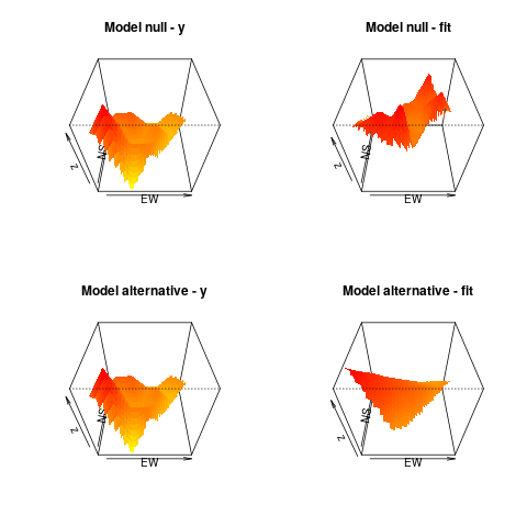
> #Plotting the estimated semivariogram from each model
> par(mfrow=c(1,2))
> Variogram(m0, main = "Semivariogram - model null", ylim = c(0,0.7))
Sill=0.098708
Practical range h=1.443974, 0.95*sill=0.093772
> Variogram(m1, main = "Semivariogram - model alternative", ylim = c(0,0.7))
Sill=0.04485
Practical range h=0, 0.95*sill=0.042608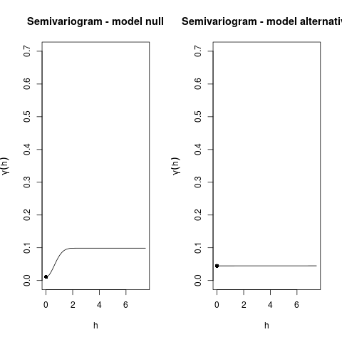
> #Summary of the estimated coefficients
> summary(m0)
            estimate std.error       t(y)  p(|t(y)|>t)    LL(95%)   UL(95%)
(Intercept)  1.19345739 0.2052892  5.8135411 1.233528e-06  0.7771115 1.6098032
B           -0.04475553 0.1458900 -0.3067759 7.607814e-01 -0.3406342 0.2511231

> summary(m1)
            estimate  std.error       t(y)  p(|t(y)|>t)     LL(95%)      UL(95%)
B            0.05574055 0.16957509  0.3287072 7.444539e-01 -0.28926256  0.400743661
(Intercept)  1.99607030 0.27884727  7.1582925 3.341973e-08  1.42875127  2.563389323
EW          -0.22207126 0.11291636 -1.9666882 5.767543e-02 -0.45180131  0.007658794
NS          -0.25988947 0.11271726 -2.3056760 2.755296e-02 -0.48921445 -0.030564487
EW.NS        0.05641610 0.03480813  1.6207739 1.145840e-01 -0.01440156  0.127233772

>
> #Some information criteria
> AIC(m0)
[1] 19.31768
> AIC(m1)
[1] 22.3003
> AICm(m0)
[1] 20.52981
> AICm(m1)
[1] 30.44845
> AICc(m0)
[1] 19.31768
> AICc(m1)
[1] 0.6983971
> BIC(m0)
[1] 25.86803
> BIC(m1)
[1] 38.67617